Arena-Based Storage Management

This is the second blog post on compiler construction. You can read the first one here.

Calling malloc incurs the obligation of a subsequent call to free which can be costly and error prone (imagine forgetting to free or freeing in-use space).

malloc allocates based on object size. I used a storage management scheme that bases allocation on object lifetime instead:

• Memory is allocated from arenas and entire arenas are deallocated at once.
• Objects with the same lifetime are allocated from the same arena.
• An arena is implemented as a linked list of contiguous blocks of memory.

The allocator acts like malloc except that it uses unsigned long instead of size_t (size_t is often defined to be unsigned int or unsigned long so we use unsigned long to account for all sizes) and takes an arena identifier from which space is allocated. The allocator returns a pointer suitably aligned to hold values of any type. A basic type is properly aligned if it is stored at an address that is a multiple of its size (this is how x86 and ARM processors lay out basic data types in memory, for example). In C, a structure gets the alignment of the member that has the widest alignment. Extra space may be allocated to account for the alignment requirements. In fact, reordering the members of a struct so that they are sorted by non-increasing alignment can reduce the memory footprint of a program significantly. You can read more about this in this excellent article by Eric Raymond: The Lost Art of C Structure Packing.

The deallocator recycles space by adding it to a list of free blocks so that the next time space needs to be allocated space from the free blocks is used. This technique renders the cost of allocation and deallocation negligible.

I recently learned that arena based storage management is used in Protocol Buffers, Google’s technology for serializing structured data.

Implementations of Algorithms and Data Structures for Competitive Programming

This is a list of algorithm and data structure implementations that can be used in competitive programming. This list is by no means exhaustive. It will grow to contain other implementations.

Data Structures

• Fenwick Trees
• Splay Trees

Graph Theory

• Lowest Common Ancestors with Binary Jumping
• Union-Find (Maintaining Disjoint Sets under Union)
• Classifying Edges in a Graph with Depth First Search
• Maximum Flow in a Flow Network

Number Theory

• Efficient Prime Factorization after Sieve
• Efficient Computation of Modular Multiplicative Inverses with (Pre-processing)

Strings and Sequences

• Longest Increasing Subsequence with Patience Sort
• Aho-Corasick
• Suffix Sort

Optimal Coloring of Chordal Graphs

How to optimally color a graph in polynomial time ? This problem is NP-complete in general but there are classes of graphs for which there exist polynomial time algorithms: trees are a very good example. In this post, we will explore a not-so-famous class of graphs: the chordal graphs. We will see that there are fast algorithms for chordal graph coloring but let us first define what chordal graphs are.

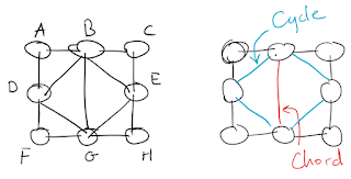
Let us assume that we are given a finite simple undirected graph $G$. $G$ is said to be a chordal graph if every induced cycle of $G$ has length 3. In other words, if $C_k, k \ge 4$ is any cycle in $G$ then $C_k$ has a chord - an edge connecting two non-consecutive vertices of the cycle. Note that by this definition every induced subgraph of $G$ is also chordal: chordality is a hereditary property. The figure to the left shows an example of a chordal graph and the figure to the right highlights a cycle of length 4 and the only chord it has.

Let us call a vertex $v$ simplicial if its neighbors, $adj(v)$, form a clique. The vertices of a chordal graph can be ordered in such a way that the kth vertex, $v_k$, is simplicial in the subgraph induced by $\{v_1, v_2, \dots, v_k\}$. Such an ordering is called a perfect elimination ordering. In fact, the chordal graphs are precisely the ones that admit a perfect elimination ordering. Once we have a perfect elimination ordering, we will be able to optimally color the graph easily.

Let us track what happens if we scan the vertices in this order and build the graph along the way. The ordering $[A, B, D, G, E, C, F, H]$ is a perfect elimination ordering of the graph above. We will shortly give an algorithm to compute such an ordering but let us see why it is useful first. The following figure shows the partial graphs that we get by adding the vertices one at a time in the ordering given above. The algorithm picks an arbitrary vertex to start with. After that, the next vertex to add is any vertex connected to a maximum number of already added vertices.

Notice that after adding a vertex $v$, then $v$ together with the vertices that are connected to it form a clique (a complete induced subgraph). The sequence of cliques that we get for this particular ordering is highlighted in yellow in the figure.

There are a few useful facts that we can extract from this example. First, a vertex adds at most one new maximal clique and so the number of maximal cliques is linear. Second, an optimal coloring contains at least as many vertices as there are in a maximum clique. We will prove that this number is sufficient.

The following algorithm for finding a perfect elimination ordering is due to Tarjan and Yannakakis; it's called maximum cardinality search, henceforth abbreviated MCS. The algorithm maintains for each vertex $v$ an integer weight, $w(v)$, which is the number of adjacent vertices whose weight is positive. All weights are set to zero initially. An implementation of this algorithm can be found here.

There are implementations that take near linear time to execute but a $O((n+m) \lg n)$ priority queue implementation will do. Now traverse the graph in that order and color (assign a number) each vertex with the smallest number not used among its predecessors. This greedy algorithm takes linear time and together with MCS gives a $O((n+m) \lg n)$ algorithm for chordal graph coloring.

The claim is that this yields an optimal coloring. To prove this we have to show that the chromatic number $\chi(G)$ coincides with the clique number $w(G)$ (not to be confused with integer weights used in the algorithm). Recall that $w(G)$ is the size of a maximum clique of $G$.

Let $indeg(v)$ denote the number of predecessors of $v$ in the ordering, i.e., the vertices adjacent to $v$ and that come earlier in the ordering. The algorithm chooses the smallest number not used among the predecessors to color the next vertex, so the minimum number of colors $\chi(G)$ is at most $\max_i\{indeg(v_i)\}+1$. Let $v_j$ be the vertex of maximum $indeg$: $\chi(G) \le indeg(v_j)+1$. Since we have a perfect elimination ordering, $v_j$ is simplicial, and $v_j$ together with its predecessors form a clique. So $w(G) \ge indeg(v_j)+1$. But we know that $\chi(G) \ge w(G)$. This implies that $\chi(G)=w(G)=indeg(v_j)+1$. This tells us that the above graph is 3-colorable for example.

We saw how to compute a perfect elimination ordering and how to use it to optimally color a chordal graph.  In fact, lots of problems that are hard on general graphs become easy on particular classes of graphs and the chordal graphs are probably the second most important class of graphs in applications. I hope that this was an enjoyable read.

Fenwick Trees

The Fenwick Tree is an elegant data structuring technique that helps solve the following problem. Given an array of numbers we would like to be able to:

• Update the element at a given position.
• Answer range sum queries.

The Fenwick tree is very easy to implement but it can be intimidating to get your head around it the first time you encounter it. This post is hopefully going to help you better understand this data structure.

Approach 1

We can use prefix sums to answer range queries in constant time but updating a position may require touching all positions in the worst case. So updates in this way are expensive.

In the usual array representation every position is responsible for itself. That is, every position remembers the value stored in it and that is it. The Fenwick Tree takes this idea of responsibility a bit further

Approach 2

We still use prefix sums but we think of each position as being responsible for a whole range ending at that position. First take a look at the diagram below. The vertical line segments are the ranges for which positions are responsible. If we take a position, write it in binary, remove all 1-bits and keep only the lowest (least significant) 1-bit then the resulting number gives the size of the range for which the position is responsible. For example, if the position is 6 (110 in binary) then the size of the range for which 6 is responsible is 2. In other words, position 6 is responsible for itself and the position before it: the range is [5..6]. Note that the size of a range is always a power of 2.

This idea of responsibility allows us to partition any prefix of the array into a union of disjoint ranges. Let's take the prefix ending at position 10 (in decimal). 10 is written as 1010 in binary. By the argument above we can say that 10 is responsible for the range [9..10]. Now we subtract the size of this range from 10 to get 8. Note that this is equivalent to removing the lowest 1-bit from 1010: 1010 becomes 1000 which is equal to 8. Now we repeat with 8 which is responsible for the range [1..8]. We remove the lowest 1-bit from 8 to get 0 and so we have partitioned the entire prefix.

The sizes of these ranges follow directly from the base-2 representation of the position. The position 10 is written as 1010 in binary, which is equal to $2^3+2^2=8+2$ and these are the ranges that we got. So nothing fancy really.

We need $\log N$ bits to represent an integer $N$ in binary, so this partitioning process takes time $O(\log N)$. This allows us to get a prefix sum in $O(\log N)$ time. Worse than the bound we got by using the first approach but this idea of responsibility is going to allow us to speed up the running time of updates.

To update a position we have to find the ranges that are responsible for it (note that a range can be represented by the position at which it ends) and update them. When a position was responsible for itself only we updated that position but now a position is responsible for itself and other positions as well.

Let us look at responsibility again. Take this bit pattern for example: 1011. If we do a query at position 1100 it gets us to position 1000 (remove lowest 1-bit) afterwards. This means that the range for which position 1100 is responsible starts at 1000 and ends at 1100. Now our bit pattern, 1011, is included in this range and so when we update position 1011 we should update 1100 as well. When we removed the lowest 1-bit from 1100 it got us to 1000 (this turned the 1 bit into a 0 and everything from 1000 to 1100 will be in the range including positions like 1011). So to get the ranges that are responsible for some position we first find the lowest 0 bit, flip it and clear all 1 bits to its right. Do the same for all 0 bits from lowest to highest. This can be simply achieved by adding the lowest 1-bit to the position each time. The ranges responsible for 1011 are: 1011, 1100, 10000, 100000, etc…

Both queries and updates require finding the lowest 1-bit. This can be done by ANDing the position with its two's complement.

• If p = 1010, p's complement is 0101 + 1 =  0110. 1010 & 0110 = 0010.

But you can come up with other methods to isolate the lowest 1-bit.

The Fenwick tree can be used to handle other types of queries. For example, range updates and point queries. With a bit more cleverness it can also be used to perform range updates and range queries. This is all for this post. I hope that it was informative.

Algorithm and Data Structure Visualizations

I started a project to help visualize algorithms and data structures. The aim is to help learners grasp the problem/algorithm by visualizing the output. The code is hosted on Github and the project is a work in progress. The Github repository will grow to contain several algorithm visualizations. The demonstrations can be accessed via this link (which also contains a link to the Github repo).

Here is a preview of some of the algorithms for which visualizations have been implemented (these include Knuth's Dancing Links, Shortest Paths, Graph Traversals, etc..):

Check regularly for updates.

Splay Trees

The standard way to achieve worst case logarithmic performance per operation in a binary search tree is by imposing a balance condition on the nodes. AVL trees, for example, force logarithmic height by making each node store its height in addition to its left/right/parent pointers. The balance condition is invariant and a rebalancing operation is necessary to restore the invariant whenever it is violated.

There is another way to obtain logarithmic performance but in an amortized sense. We do not need to impose a balance condition. Rather, the tree adjusts itself after each operation by using a restructuring heuristic. Sleator and Tarjan proposed a heuristic that achieves O(lg n) time amortized per operation (over a sequence of operations). This heuristic is the splay operation. In the remainder of this post, we shall describe how the splay operation works and provide a C/C++ implementation.

We are going to use a C++ structure to represent a node. A node stores pointers to its left/right children and to its parent. Initially, all pointers point to nothing.

In a splay tree, a node x is splayed to the root of the tree whenever it is accessed. Splaying x works by climbing the x-to-root path by following parent pointers and performing rotations. A rotation is a local restructuring operation. If x is a left child, it is rotated to the right and if it is a right child, it is rotated to the left. The following is a pictorial representation of a rotation. Here x and y are nodes and A, B and C are sub-trees (possibly null).

Rotations do not change the binary search property, i.e., inorder traversals of the tree before and after the rotation give the same output. The following function performs a right rotation.

Here is code to perform a left rotation.

The splay operation performs rotations in pairs. There are two cases to consider, a zig-zig case and a zig-zag case. Let x be the node that we want to splay and let y be its parent. The zig-zig case occurs when both x and y are left children (or both right children). The zig-zag case occurs when x is a left child and y is a right child (or x is a right child and y is a left child). If y is neither a left nor a right child (it is the root), we do a single rotation. Let us elaborate.

The following figure shows the pair of rotations performed in the zig-zig step. Here x is a left child and y is a left child (the right-right case is symmetric). The order of rotations is important, we first rotate y and then we rotate x.

The following figure shows the pair of rotations performed in the zig-zag step. Here x is a right child and y is a left child (the left-right case is symmetric). We rotate x twice

To wrap, there are two cases up to symmetry and four cases in general, and we might do one last rotation at the end if x does not have a grand-parent.

By the end of the splay operation, x becomes the root of the tree. This is very useful because nodes that are accessed frequently live near the root of the tree as a result of splay.

Now you can augment nodes with keys and use the splay operation to implement the other operations. For example, to insert a node with key k, you do a regular binary search on k to find where to insert the node, and then you splay that node to the root of the tree.

That is all for this post. Thank you for reading !

I am Writing a Compiler for C in C

First day of the adventure: I really want to finish this work. I started reading ‘A retargetable C compiler: design and implementation’ to learn the tricks of the trade and I will commit to finishing the implementation of a working ISO C compiler. Along the way I will be taking notes and writing about the experience.

In the past, I wrote independent components of compilers but never finished a complete compiler. This was due to lack of motivation/resources and partially because I teamed up with other people without having a clear picture in mind of who was doing what and how. I decided that this project is going to be a solo adventure.

Why learn how to build a C compiler ?

• Only few programmers know how to build compilers. They are better programmers and better C programmers.
• The compiler writer must understand even the darkest corners of the C programming language. This reveals much about the language itself.
• A compiler is one of the best demonstrations of the interactions between theory and practice. Writing a compiler helps understand where these interactions are smooth and elegant and where practical demands strain the theory.

A compiler translates source code to assembler or object code for a target machine. A retargetable compiler has multiple targets.

The book focuses on the implementation of a retargetable compiler for three target machines. I will lower expectations this time and shoot for one target: the x86 architecture. The book also cares less about theory and describes only the bits of theory needed for the actual implementation. I have read a lot about theory so the lack of theory coverage will go unnoticed.

Design goals:

• Fast scanner and instruction selector.
• Generate code of reasonable quality.
• Machine independent optimizer (local optimization).
• Hand-crafted scanner and parser (recursive).
• Clean semantic checker.

This is all for this post. I will be sharing code gradually.

Heuristic Inverse Kinematics with FABRIK

Inverse kinematics (IK for short) is the problem of computing end-positions for a chain of joints . FABRIK is a heuristic technique for solving an IK system. In the figure below, the joint $p_0$ is fixed and the joint $p_n$ is free. $p_n$ is also called an end-effector. We would like to be able to move the end-effector freely and the system should compute locations for the joints $p_1,\dots,p_{n}$ so that the end-effector reaches a target position. Think of it as a robotic arm trying to reach a target.

[figure]

Before describing the technique, I invite you to watch this demo FABRIK solver that I created.

There are several ways to solve an IK system. Some give exact solutions but require a lot of time to calculate the joint positions; these are preferred techniques when precision matters. If you are going to write a simulation or an IK solver for a video game, for example, then you might consider using FABRIK; the results are by far the best in terms of realism and the algorithm is very fast.

The overall idea is simple. We iteratively improve upon the current joint positions until the distance between the end-effector and the target position is good enough. We also set an upper-bound on the number of iterations (this is a small number in practice) to avoid looping forever.

In a single iteration we perform a forward pass in which the joints get closer to the target (this shifts the fixed joint as well) and a backwards pass in which the joints get closer to the fixed joint (this gets the fixed joint back to its position). After every iteration, the calculated new joint positions are improved. How are the new joint positions calculated ? This is where the heuristic part comes in.