How to optimally color a graph in polynomial time ? This problem is NP-complete in general but there are classes of graphs for which there exist polynomial time algorithms: trees are a very good example. In this post, we will explore a not-so-famous class of graphs: the chordal graphs. We will see that there are fast algorithms for chordal graph coloring but let us first define what chordal graphs are.
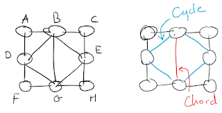
Let us assume that we are given a finite simple undirected graph $G$. $G$ is said to be a chordal graph if every induced cycle of $G$ has length 3. In other words, if $C_k, k \ge 4$ is any cycle in $G$ then $C_k$ has a chord - an edge connecting two non-consecutive vertices of the cycle. Note that by this definition every induced subgraph of $G$ is also chordal: chordality is a hereditary property. The figure to the left shows an example of a chordal graph and the figure to the right highlights a cycle of length 4 and the only chord it has.
Let us call a vertex $v$ simplicial if its neighbors, $adj(v)$, form a clique. The vertices of a chordal graph can be ordered in such a way that the kth vertex, $v_k$, is simplicial in the subgraph induced by $\{v_1, v_2, \dots, v_k\}$. Such an ordering is called a perfect elimination ordering. In fact, the chordal graphs are precisely the ones that admit a perfect elimination ordering. Once we have a perfect elimination ordering, we will be able to optimally color the graph easily.

Let us call a vertex $v$ simplicial if its neighbors, $adj(v)$, form a clique. The vertices of a chordal graph can be ordered in such a way that the kth vertex, $v_k$, is simplicial in the subgraph induced by $\{v_1, v_2, \dots, v_k\}$. Such an ordering is called a perfect elimination ordering. In fact, the chordal graphs are precisely the ones that admit a perfect elimination ordering. Once we have a perfect elimination ordering, we will be able to optimally color the graph easily.
Let us track what happens if we scan the vertices in this order and build the graph along the way. The ordering $[A, B, D, G, E, C, F, H]$ is a perfect elimination ordering of the graph above. We will shortly give an algorithm to compute such an ordering but let us see why it is useful first. The following figure shows the partial graphs that we get by adding the vertices one at a time in the ordering given above. The algorithm picks an arbitrary vertex to start with. After that, the next vertex to add is any vertex connected to a maximum number of already added vertices.

Notice that after adding a vertex $v$, then $v$ together with the vertices that are connected to it form a clique (a complete induced subgraph). The sequence of cliques that we get for this particular ordering is highlighted in yellow in the figure.
There are a few useful facts that we can extract from this example. First, a vertex adds at most one new maximal clique and so the number of maximal cliques is linear. Second, an optimal coloring contains at least as many vertices as there are in a maximum clique. We will prove that this number is sufficient.
The following algorithm for finding a perfect elimination ordering is due to Tarjan and Yannakakis; it's called maximum cardinality search, henceforth abbreviated MCS. The algorithm maintains for each vertex $v$ an integer weight, $w(v)$, which is the number of adjacent vertices whose weight is positive. All weights are set to zero initially. An implementation of this algorithm can be found here.
There are implementations that take near linear time to execute but a $O((n+m) \lg n)$ priority queue implementation will do. Now traverse the graph in that order and color (assign a number) each vertex with the smallest number not used among its predecessors. This greedy algorithm takes linear time and together with MCS gives a $O((n+m) \lg n)$ algorithm for chordal graph coloring.
The claim is that this yields an optimal coloring. To prove this we have to show that the chromatic number $\chi(G)$ coincides with the clique number $w(G)$ (not to be confused with integer weights used in the algorithm). Recall that $w(G)$ is the size of a maximum clique of $G$.
Let $indeg(v)$ denote the number of predecessors of $v$ in the ordering, i.e., the vertices adjacent to $v$ and that come earlier in the ordering. The algorithm chooses the smallest number not used among the predecessors to color the next vertex, so the minimum number of colors $\chi(G)$ is at most $\max_i\{indeg(v_i)\}+1$. Let $v_j$ be the vertex of maximum $indeg$: $\chi(G) \le indeg(v_j)+1$. Since we have a perfect elimination ordering, $v_j$ is simplicial, and $v_j$ together with its predecessors form a clique. So $w(G) \ge indeg(v_j)+1$. But we know that $\chi(G) \ge w(G)$. This implies that $\chi(G)=w(G)=indeg(v_j)+1$. This tells us that the above graph is 3-colorable for example.
We saw how to compute a perfect elimination ordering and how to use it to optimally color a chordal graph. In fact, lots of problems that are hard on general graphs become easy on particular classes of graphs and the chordal graphs are probably the second most important class of graphs in applications. I hope that this was an enjoyable read.